Pressure drop in thin perforated plates
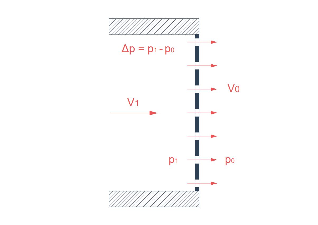
( \zeta ) (or K) is defined as the pressure drop coefficient by the fundamental equation:
\zeta = \Large \frac {\Delta p}{\frac{1}{2} \rho V_1^2}
Where:
- \Delta p : pressure drop across the plate [Pa].
- V_1 : approach velocity of the air before the plate [m/s].
- \rho : air density [kg/m³].
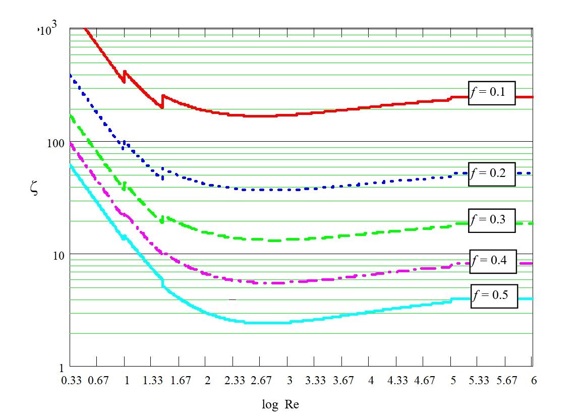
The pressure drop coefficient ( \zeta ) is a function of the free area ratio or porosity ( f ) and the Reynolds number ( Re ). Porosity ( f ) varies between 0 (closed) and 1 (fully open).
To characterize the flow regime, we calculate the Reynolds number based on the orifice diameter:
Re = \Large \frac{V_0 d_h}{\nu}
Where:
- V_0 : fluid velocity inside the orifice [m/s].
- d_h : hydraulic diameter of the orifice [m].
- \nu : kinematic viscosity [m²/s].
| Regime | Reynolds | ζ |
|---|---|---|
| Turbulent | Re ≥ 1000 | ζ= ζ (diag.1-2) |
| Transitional | 10 ≤ Re ≤ 1000 | |
| Laminar | Re ≤ 10 | ζ = 30/(f² Re) |
Using the continuity equation ( f V_0 = V_1 ), we can express the Reynolds number as a function of the approach velocity, which is easier to measure in ducts:
Re = \Large \frac{V_1 d_h}{f \nu}
Depending on the Reynolds number ( Re ), the flow behaves differently. This is critical for accurate simulation, since the coefficient \zeta is not constant across all regimes.
From Paper to Simulation: The Porous Media Model
In CFD software like Ansys Fluent or OpenFOAM, perforated plates are often modeled as “Porous Media” or “Cell Zones” to save computational cost. The software uses the Darcy-Forchheimer equation, which relates the pressure gradient to velocity using two distinct resistance coefficients:
\large\frac{\Delta p}{L}\normalsize = \underbrace{\frac{\mu}{\alpha} v}_{\text{Viscous}} + \underbrace{C_2 \frac{1}{2} \rho v^2}_{\text{Inertial}}
The dimensionless pressure drop coefficient (ζ or K) can also be related to the porous media model coefficients (α and C_2 ) required by Ansys Fluent or OpenFOAM.
K = \underbrace{ \frac{2 \mu L}{\alpha \rho} \cdot \frac{1}{v} }_{\text{Viscous}} + \underbrace{ C_2 L }_{\text{Inertial}}
Where:
- K : pressure drop coefficient (Dimensionless).
- L : thickness of the plate or porous medium [m].
- \alpha : permeability [m²].
- C_2 : inertial resistance coefficient [m⁻¹].
- \mu : dynamic viscosity [Pa·s].
- \rho : fluid density [kg/m³].
- v : fluid velocity [m/s].
- Laminar Regime (Re < 10): The Viscous Term (1/α)
At low velocities, the viscous term dominates. The pressure drop is linear (\Delta p \propto v). In this region, \zeta drops rapidly as the Reynolds number increases. In Ansys, this is controlled by the Viscous Resistance (1/α).
- Turbulent Regime (Re > 1000): The Inertial Term (C_2)
At high velocities, inertial forces dominate. The pressure drop becomes quadratic (\Delta p \propto v^2) and \zeta becomes constant. In Ansys, this is controlled by the Inertial Resistance (C_2).
- The Critical Transition Zone (Re ≈ 10 – 1000)
Most industrial ventilation and filtration systems operate in this range. Here, neither term is negligible. Standard formulas often fail because \zeta is a complex curve that depends on both viscosity and geometry.
To simulate this accurately, at Atreydes Engineering we calculate both coefficients (1/\alpha and C_2) to reconstruct the exact pressure drop curve for your specific fluid and geometry.
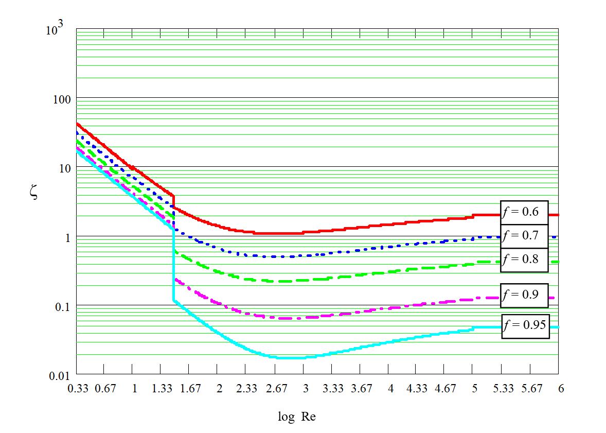
The following diagrams (double logarithmic scale) show the empirical behavior of \zeta used to calibrate these CFD models:
Do you need accurate pressure drop calculations?
Stop relying on approximations for critical equipment. We simulate the exact geometry of your perforated plate using advanced CFD to determine the precise hydraulic resistance.