Fatigue

Often, machine members are found to have failed under the action of repeated or
fluctuating stresses; yet the most careful analysis reveals that the actual maximum
stresses were well below the ultimate strength of the material, and quite frequently even
below the yield strength. The most distinguishing characteristic of these failures is that
the stresses have been repeated a very large number of times. Hence this failure is called
a fatigue failure.

Fatigue failure is due to crack formation and propagation. A fatigue crack will typically initiate at a discontinuity in the material where the cyclic stress is a maximum.

The rate and direction of fatigue crack propagation is primarily controlled by localized stresses and by the structure of the material at the crack. However, as with crack formation, other factors may exert a significant influence, such as environment, temperature, and frequency. As stated earlier, cracks will grow along planes normal to the maximum tensile stresses. The crack growth process can be explained by fracture mechanics.

Shigley’s Mechanical Engineering Design

In this section, we will focus on fatigue calculation by means of the stress-life method, which tries to extrapolate the results obtained from laboratory tests to components in real applications. It should be taken into account that although this method has traditionally been used in engineering, it is not the most accurate, so the calculations obtained should be considered as an approximation of the behavior in reality. The only way to know exactly the fatigue performance of an element is to test it under the cyclic loads to which it will be subjected. The formulation presented in these sections refers to ferrous materials (steels) which are known to have an infinite life at high numbers of cycles ( $10^6$ ) for a given load. This is not the case for other materials such as aluminum, which always undergoes a downward curve, so that a fatigue load value is usually given for $5\cdot10^8$ cycles.

The Endurance Limit (Se)

The Endurace Limit (Se)

According to different steel tests, the endurance limit ( $S_e'$ ) can be estimated through the ultimate tensile strength ( $S_{ut}$ ) as follows:

$S_e' = \begin{cases} 0.5 S_{ut} &\text{si } S_{ut} \le 200 kpsi \\ 100 kpsi & \text{si } S_{ut} > 200 kpsi \end{cases}$

The endurance limit must be modified to adapt to the conditions of our actual application, so Marin equation is used, which takes into account several factors:

$S_e = k_a \cdot k_b \cdot k_c \cdot k_d \cdot k_e \cdot k_f \cdot S_e'$

Surface factor (ka)

This factor depends on the surface finish quality of the component and its tensile strength.

$k_a = a S_{ut}^b$

The values of "a" and "b" are shown in the following table:

Surface finish (Acabado superficial)	Factor a	Exponent b
Ground (Esmerilado)	1.34	-0.085
Machined (Mecanizado)	2.70	-0.265
Cold-drawn (Laminado en frio)	2.70	-0.265
Hot-rolled (Laminado en caliente)	14.4	-0.718
As-forged (Forja)	39.9	-0.995

Size factor (kb)

The bending and torsion results can be expressed as follows:

$k_b = \begin{cases} 0.879d^{-0.107} &\text{para } 0.11 \le d \le 2 in \\ 0.91d^{-0.157} & \text{para } 2 < d \le 10 in \end{cases}$

There is no size effect for axial loading, so:

$k_b = 1$

For non-circular rotating or static cross-sections, it is necessary to compare the area that supports a stress equal to or greater than 95% of the maximum stress with the area of the circular rotating section in order to obtain an equivalent diameter (de) to substitute in the equalities described above. For a circular or annular rotating section, d = de:

$A_{0.95\sigma} = \Large \frac {\pi}{4} \normalsize [d^21 - (0.95d)^2] = 0.0766d^2 = 0.0766d_e^2$

A table for structural cross-sections is included:

Sección	A0.95σ	de
Circular o anular estática de diámetro d	0.01046d²	0.370d
Rectangular maciza o hueca rotativa de lados b x h	0.0975hb	1.128(hb)^(½)
Rectangular maciza o hueca estática de lados b x h	0.05hb	0.808(hb)^(½)

Loading factor (kc)

When fatigue tests are performed with rotary, axial and torsional bending loads, the endurance limits differ with Sut.

$k_c = \begin{cases} 1 &\text{flexión } \\ 0.85 & \text{axial } \\ 0.59 & \text{torsión } \end{cases}$

Temperature factor (kd)

When operating temperatures are below room temperature, brittle fracture is a strong
possibility and should be investigated first. When the operating temperatures are higher
than room temperature, yielding should be investigated first because the yield
strength drops off so rapidly with temperature.

$k_d = \small 0.975 + 0.432\cdot 10^{-3} T_F - 0.115\cdot 10^{-5} T_F^2 + 0.104\cdot 10^{-8} T_F^3 - 0.595\cdot 10^{-12} T_F^4$

For 70 ≤ $T_F$ ≤ 1000 ºF

Reliability factor (ke)

To take into account for data dispersion. Most of these data are reported as mean values with a standard deviation of 8%. A table relating reliability to the reliability factor (ke) is shown below.

Confiabilidad (%)	ke
50	1
90	0.897
95	0.868
99	0.814
99.9	0.753
99.99	0.702
99.999	0.659
99.9999	0.620

Miscellaneous-Effects factor (kf)

Though the factor kf is intended to account for the reduction in endurance limit due to all other effects, it is really intended as a reminder that these must be accounted for, because actual values of kf are not always available.

Some of these factors that can be decisive in the endurance limit are:

Residual Stresses

Corrosion

Electrolytic plating

Metal spraying

Cyclic Frequency

Frettage corrosion

Chart S-N

Traditionally fatigue tests and later extrapolations for components in real applications have been plotted on S-N charts in the logarithmic plane.

It should be mentioned that these graphs are only valid for a single completely reversed stress, i.e., it fluctuates from a maximum to a minimum with average equal to zero, so the maximum and minimum are equal and with opposite sign.

Gráficas S-N

The two negative slopes follow the next equation:

S_f = a N^b

N = \left( \Large \frac{S_f}{a} \right)^{\large \frac{1}{b}}

Where the factor "a" and the exponent "b" take the following values:

For the first slope:

a = S_{ut}

b = - \Large \frac{1}{3}\normalsize \log \left(\Large \frac{1}{f} \right)

And for the second slope:

a = \Large \frac{(f S_{ut})^2}{S_e}

b = - \Large \frac{1}{3}\normalsize \log \left(\Large \frac{(f S_{ut})^2}{S_e} \right)

Where

f

is a fraction of

S_{ut}

f = \Large \frac {\sigma_F'}{S_{ut}} \normalsize (2\cdot 10^3)^c

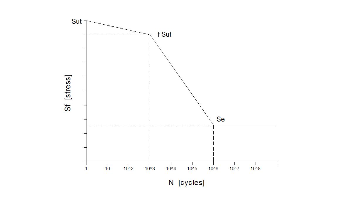
With the SAE approach for steel with $H_B \le$ 500:

$\sigma_F' = S_{ut} + 50 kpsi$

And with “b”:

$c = - \Large \frac {log (\sigma_F' / S_{e}')}{log (2\cdot 10^6)}$

Where $S_e'$ is the endurance limit without modifications.

Stress Concentration (Kf)

The existence of irregularities or discontinuities, such as holes, slots or notches significantly increases the theoretical stresses in the immediate vicinity of the discontinuity. This increase, which is defined by the stress concentration factor (Kt), is related to its counterpart in fatigue analysis (Kf) through Neuber equation:

$K_f = 1+ \Large \frac {K_t - 1}{1 + \frac{\sqrt{a}}{\sqrt{r}}}$

Where $\sqrt {a}$ is Neuber constant whose value for bending and axial stresses is:

$\sqrt{a} = 0.246 - 3.08 \cdot 10^{-3} S_{ut} + 1.51 \cdot 10^{-5} S_{ut}^2 - 2.67 \cdot 10^{-8} S_{ut}^3$

And for torsional stress:

$\sqrt{a} = 0.190 - 2.51 \cdot 10^{-3} S_{ut} + 1.35 \cdot 10^{-5} S_{ut}^2 - 2.67 \cdot 10^{-8} S_{ut}^3$

Where the equations apply to steel, $S_{ut}$ is in kpsi and “r” is the notch radius in inches (in).

Tables of theoretical values of the concentration factor (Kt) are shown below.

Concentration-factors-Kt

Fluctuating Stresses

Fluctuating stresses in machinery often take the form of a sinusoidal pattern because of the nature of some rotating machinery. However, other patterns, some quite irregular, do occur. It has been found that in periodic patterns exhibiting a single maximum and a single minimum of force, the shape of the wave is not important, but the peaks on both the high side (maximum) and the low side (minimum) are important.

Fluctuating Stresses

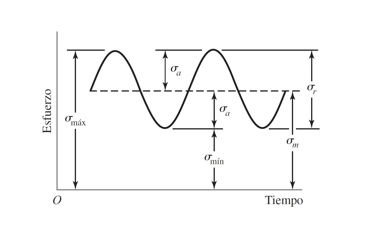
$\sigma_{min}$ = minimum stress

$\sigma_{max}$ = maximum stress

$\sigma_{m}$ = midrange component

$\sigma_{a}$ = amplitude component

$\sigma_{r}$ = range of stress

$\sigma_m = \Large \frac {\sigma_{max} + \sigma_{min}}{2}$

$\sigma_a = \Large | \frac {\sigma_{max} - \sigma_{min}}{2}|$

Fatigue failure criteria

The following criteria are representative for ductile materials with creep zones. For brittle steels, such as cast iron, they follow the concave and upward Smith-Dolan model.

Fatigue failure criteria

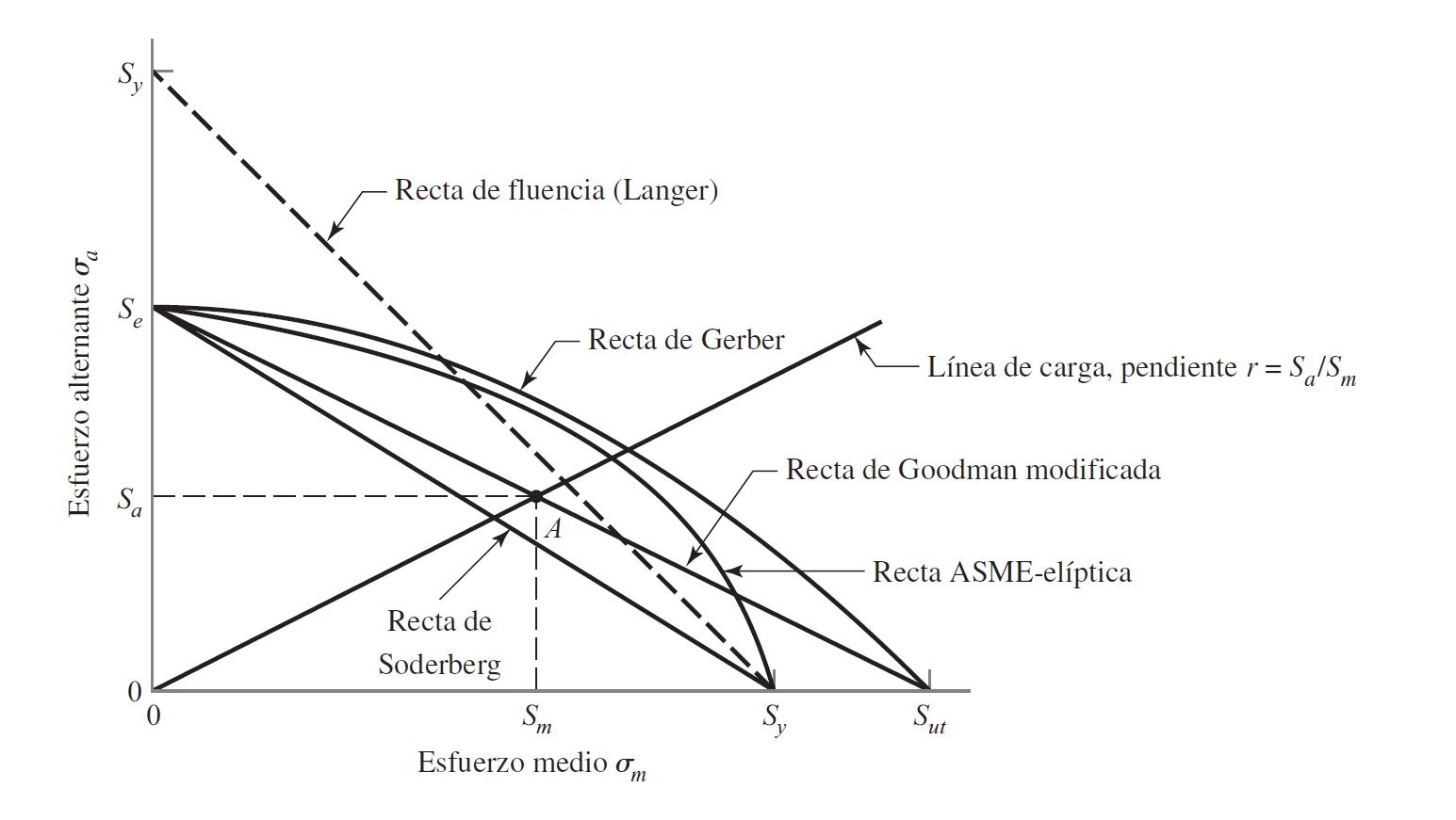
Soderberg

$\Large \frac{S_a}{S_e}\normalsize + \Large \frac{S_m}{S_y} \normalsize = 1$

Mod-Goodman

$\Large \frac{S_a}{S_e}\normalsize + \Large \frac{S_m}{S_{ut}} \normalsize = 1$

Gerber

$\Large \frac{S_a}{S_e}\normalsize + \Large (\frac{S_m}{S_{ut}})\normalsize^2 = 1$

ASME-elíptica

$\Large (\frac{S_a}{S_e})\normalsize^2 + \Large (\frac{S_m}{S_y})\normalsize^2 = 1$

Langer static yield

$S_a+ S_m = S_y$

The two most commonly used criteria are Gerber and ASME-elliptic. The Sorderberg and Goodman criteria continue to be retained for their simplicity, since both describe a straight line. The Langer criterion, which describes the static case, is also added.

Failure criteria are used together with the load line $r = S_a/S_m = \sigma_a/\sigma_m$ .

The intersection of the Gerber and ASME-elliptic criteria with the load line (r), together with its safety coefficient (nf), is shown below:

Gerber

$S_a = \Large \frac{r^2S_{ut}^2}{2S_e} \left [\normalsize-1+\sqrt{1+ \left(\Large \frac{2S_e}{r S_{ut}} \right)^2} \right]$

$S_m = \Large \frac{S_a}{r}$

$n_f = \Large \frac{1}{2} \normalsize \left( \Large \frac{S_{ut}}{S_m} \right)^2 \Large \frac{S_{a}}{S_e} \normalsize \left[ -1+\sqrt{1+ \left(\Large \frac{2 S_m S_e}{S_a S_{ut}}\right)^2}\right]$

ASME-elíptica

$S_a = \sqrt{\Large \frac{r^2 S_e^2 S_y^2 }{S_e^2 + r^2 S_y^2}}$

$S_m = \Large \frac{S_a}{r}$

$n_f = \sqrt{\Large \frac{1}{(S_a / S_e)^2 + (S_m / S_y)^2}}$

Varying and fluctuating stresses

When we have varying and fluctuating stresses, it is very important to identify all the cycles in the time series, since some of them may be hidden. We can see in the figure the identification of 3 cycles that repeat over time. When initially two had been defined, the displacement in stresses of the first one with respect to the second one finds a hidden cycle of greater magnitude than the other two previous ones, which will be the determining factor for the fatigue design.

Varying and fluctuating stresses

The stress parameters of these three cycles are shown below:

nº cycle	σmax	σmin	σa	σm	r = σa/σm
1	80	-60	70	10	7
2	60	40	10	50	0.2
3	-20	-40	10	-30	-0.333

The fatigue contribution of each of these cycles (ni) must be calculated individually, weighted by an equivalent number of cycles (Neq) in Miner formulation of the accumulated damage (D).

$D = \sum_{i=1}^n N_{eq} \left(\Large \frac{1}{n_i} \right)$

In Miner formulation, fatigue failure occurs when the accumulated damage (D) is greater than or equal to 1.

Load Combinations

When axial, bending and torsional forces are present, Von Mises stress is calculated for $\sigma_{m}'$ and $\sigma_{a}'$ as follows:

$\sigma_m' = \sqrt{ \left[ (K_f)_{fl} (\sigma_m)_{fl} + (K_f)_{ax} (\sigma_m)_{ax} \right]^2 +3 \left[ (K_f)_{tor} (\tau_m)_{tor} \right]^2 }$

$\sigma_a' = \sqrt{ \left[ (K_f)_{fl} (\sigma_a)_{fl} + (K_f)_{ax} (\sigma_a)_{ax} \right]^2 +3 \left[ (K_f)_{tor} (\tau_a)_{tor} \right]^2 }$

Once Von Mises stresses $\sigma_{m}'$ and $\sigma_{a}'$ have been calculated, they can be entered into the fatigue criteria already defined:

If the stress components are not in phase but have the same frequency, the maxima
can be found by expressing each component in trigonometric terms, using phase angles,
and then finding the sum. If two or more stress components have differing frequencies,
the problem is difficult; one solution is to assume that the two (or more) components
often reach an in-phase condition, so that their magnitudes are additive

Accumulated Damage

Once a component has received fatigue damage without reaching failure, its S-N curve must be modified according to the remaining damage it has yet to receive.

The example chart shows the S-N curve of a component (continuous curve) and its modification (dashed curve) after application of a reversed load of $\sigma_1$ = 60 kpsi with a number of cycles of $3 \cdot 10^3$ .

Accumulated damage

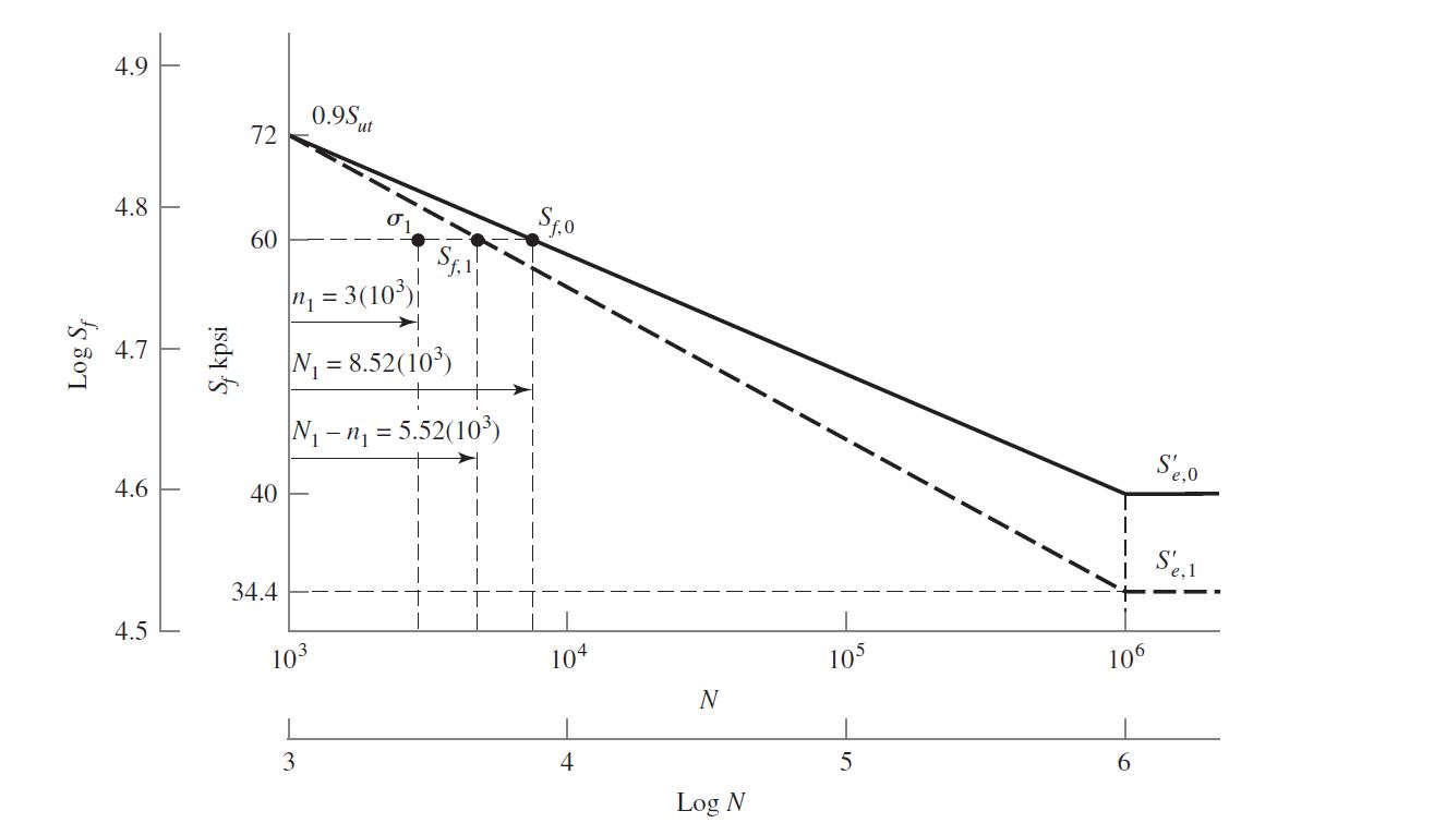
Since insufficient numbers of cycles ( $N_1$ ) occur to produce fatigue damage, the component can still resist fatigue but its curve must be modified since it has accumulated the damage from the described loading.

For this purpose, a new descending line is drawn through the point $(N_1-n_1, \sigma_1)$ to the new endurance limit $S_{e,1}'$ at $10^6$ cycles.

This modification changes the endurance limit level of the component so that it is no longer able to withstand the same load at infinite time.

(+34) 605 304 564

Fatigue

Handbooks

Services

Projects

About Us

Downloads

Fatigue

The Endurace Limit (Se)

Surface factor (ka)

Size factor (kb)

Loading factor (kc)

Temperature factor (kd)

Reliability factor (ke)

Miscellaneous-Effects factor (kf)

Residual Stresses

Corrosion

Electrolytic plating

Metal spraying

Cyclic Frequency

Frettage corrosion

Chart S-N

Stress Concentration (Kf)

Fluctuating Stresses

Fatigue failure criteria

Soderberg

Mod-Goodman

Gerber

ASME-elíptica

Langer static yield

Gerber

ASME-elíptica

Varying and fluctuating stresses

Load Combinations

Accumulated Damage

Contact

Centro de Negocios INN Offices Sevilla Cartuja. Calle Leonardo da Vinci, 20. Parque Científico y Tecnológico Cartuja, 41092 Seville (Spain) [shortly]

(+34) 605 304 564

Extra links