Projects


About Us

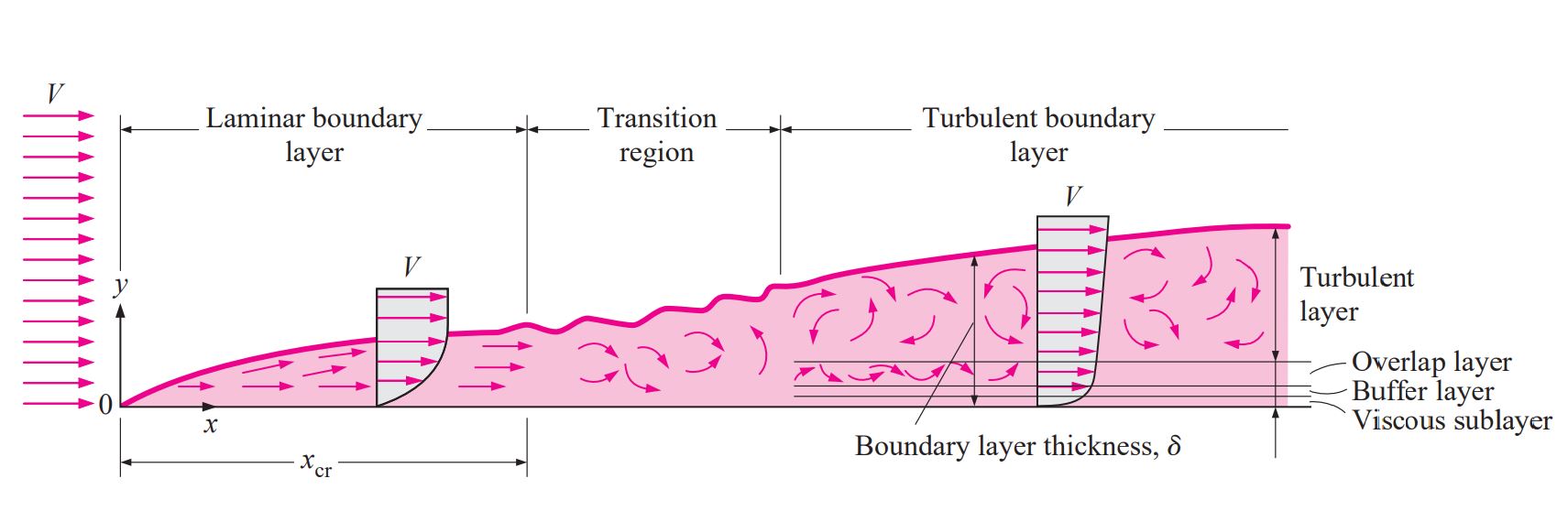
Turbulent Flow
Y+ parameter
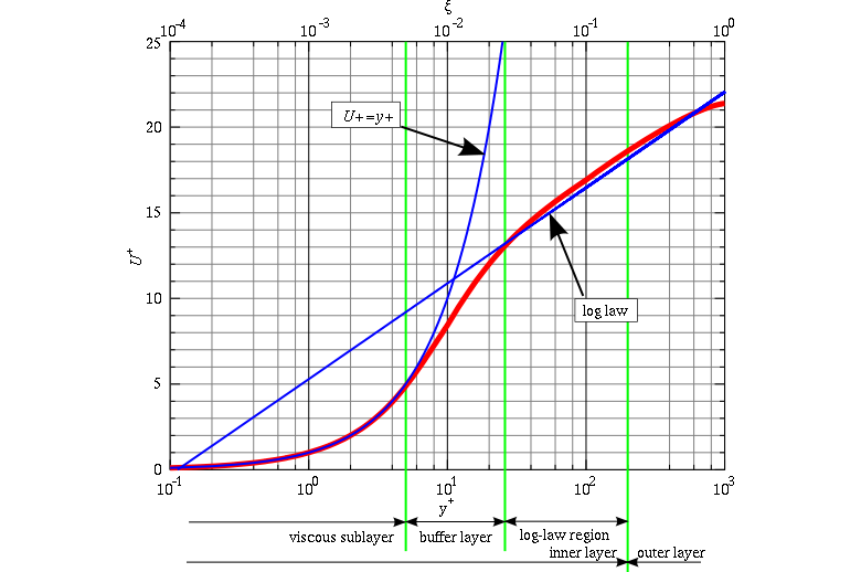
Y+ calculation
y_p= \Large \frac {y^+ \mu} {u_{\tau} \rho}
y_H= 2 y^+
The friction velocity ( u_{\tau} ) is calculated as:
u_{\tau} = \sqrt{ \Large \frac {\tau_{\omega}} {\rho}}
Where wall shear stress ( \tau_{\omega} ) depends on the skin friction coefficient ( C_f):
\tau_{\omega} = \Large \frac {1}{2}\normalsize \rho U^2 C_f
Where U is the free stream velocity of the fluid and the skin friction coefficient ( C_f ) must be estimated since we do not know it, so we will take the flat plate one in turbulent regime.
C_f = (2 \log_{10} (Re) - 0.65)^{-2.3}
For internal flows: C_f= 0.079 Re^{-0.25}
For external flows: C_f= 0.058 Re^{-0.2}
Re = \Large \frac {\rho U L} {\mu}
Turbulence coefficients
k = \Large \frac {3} {2} \normalsize U^2 I^2
If the maximum free stream velocity is defined as U_{max} , then the turbulence intensity (I) is calculated as:
I (\%) = \Large \frac {U_{max}-U} {U} \normalsize \cdot 100 = (G-1)\cdot 100
U_{max} = G \cdot U
\epsilon = C_{\mu} \Large \frac {\rho k^2}{\mu} \normalsize \beta^{-1}
Where C_{\mu} = 0.09 in the methods k-ϵ and k-ω, and β is the turbulent viscosity ratio.
\beta = \Large \frac{\mu_t}{\mu}
\omega = \Large \frac {\rho k}{\mu} \normalsize \beta^{-1}
| Turbulence | Re | I (%) | β |
|---|---|---|---|
| Very low | 0.05-1 | 0.1-0.2 | |
| Low | 3000-5000 | 1 | 11.6-16.5 |
| Medium | 5000-15000 | 1-5 | 16.5-26.7 |
| High | 15000-20000 | 5-20 | 26.7-34 |
| Very high | >50000 | 100 |
1< \beta < 10