Fluttering design process of solar trackers
We describe the fluttering design process that relates the most important variables involved in aeroelastic phenomena as well as the components of a single-axis tracker which are affected by or support the loads of these instabilities.
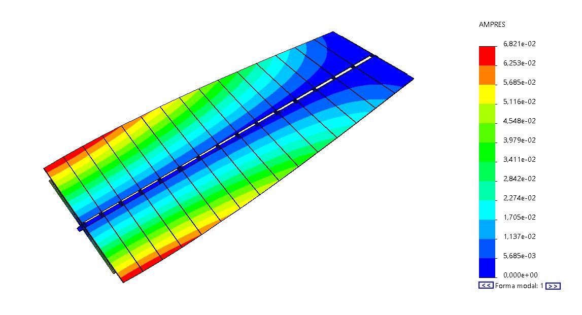
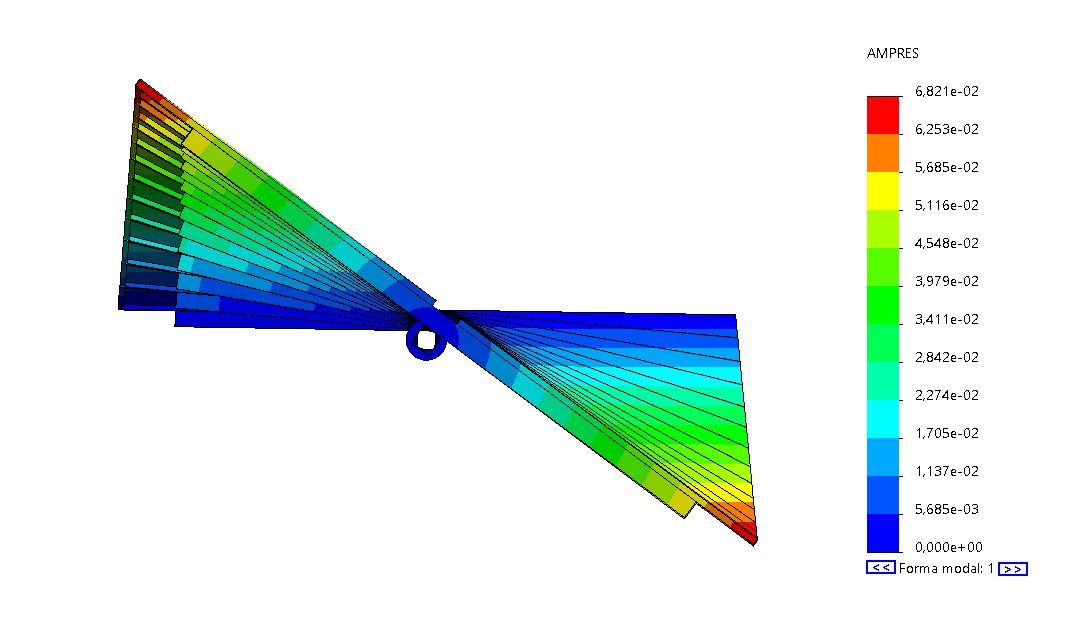
Before starting with the aeroelastic calculation process, it is necessary to have define the tracker geometry which will provide us with its natural frequency (n) and its associated vibration mode:
| Material | Yield Limit [MPa] |
|---|---|
| S275JR | 250 |
| S355JR | 320 |
-
- Static limit (holding torque) or maximum value of torque loads it can withstand completely stopped.
-
- Nominal dynamic limit (nominal torque) or nominal value that it can maintain when moving. This value must be associated with average wind speeds ( V_{1h} ).
-
- Maximum dynamic limit (maximum torque) or maximum value that it can maintain for a short instant of time, normally considered for 3 seconds, so it is compared with the maximum peak wind speed ( V_{3s} ) that is reached instantaneously for a given average wind speed ( V_{1h} ).
Any mechanism supports more load when idle than when in motion. The ratio between the static limit and the maximum dynamic one is usually between 2 and 3.
For this geometry, a natural frequency of 2.1Hz is obtained which provides the torsional mode of vibration.
To fully check the torsional loads on the tracker components, it is necessary to take into account the torsional moments due to the weight offset introduced by the photovoltaic modules when they are tilted by the tracker operating motion. So, the torsion will be given by the action of the wind load plus the moment provided by the weight of the tracker itself.
Aeroelastic phenomena introduce mainly tangential stresses ( \tau_t ) due to torsional moments ( M ), but drag and lift loads due to wind forces ( F ) will produce bending normal stresses ( \sigma_b ) and shear tangential stresses ( \tau_c ) which, although smaller than the torsional ones ( \tau_t ), must be computed according to the Von Mises formula ( \sigma_{VM} ) to obtain the total stress on the tracker components.
\sigma_{VM} = \sqrt{\sigma_b^2 + 3 (\tau_t + \tau_c)^2}
Two-dimensional vs three-dimensional models
Fluttering design process is based on a two-dimensional model in which only the distortion or twist of the tracker last section is taken into account. Since the mode of vibration is a tracker linear torsion, the twist of the other sections can be known by their distance to the last section given that the torque tube total length is also known. The two-dimensional parameters of inertia ( I ) and stiffness ( k ) should not be confused with the three-dimensional ones, which we will call \hat I and \hat k to distinguish them.
Given the distortion of the tracker last section in the three-dimensional model when a linearly distributed moment is applied to it, the values of inertia ( I ) and stiffness ( k ) can be adjusted to achieve the same rotation for the same load, this time per meter, in the two-dimensional model.
The stiffness of a three-dimensional system ( \hat k ) can be defined as:
\hat k = (2\pi n)^2 \hat I
Where n is the natural frequency of the torsional mode of vibration and \hat I is the three-dimensional inertia in the torsional axis usually obtained from design software (CAD). Design software provide the rotational inertia of the entire structure with respect to the vibration mode axis ( \hat I_{cad} ), but do not calculate the inertia contributing to this mode. It is also known that the inertia contributing to a torsional mode of vibration with one of the ends fixed is one third of the structure inertia if it rotates with both ends free so:
\hat I = \Large \frac{1}{3} \normalsize \hat I_{cad}
Writing again the stiffness, but this time with inertia provided by a design software, we have that:
\hat k = \Large \frac{1}{3} \normalsize (2\pi n)^2 \hat I_{cad}
On the other hand, we can make an approximation of the two-dimensional stiffness (k) and inertia (I) through the last section rotation of the three-dimensional tracker with a linearly distributed load (m).
\theta_{ 3d} = \theta_{ 2d}
\Large \frac{1}{2} \frac{m L^2}{GJ} \normalsize = \Large \frac{m}{k}
Where stiffness (k) is equal to:
k = \Large \frac{2GJ}{L^2}
Siendo:
- G: material shear modulus
- J: torsional constant for the section
- L: torque tube length
These formulas are approximate, since it is being taken into account that the tracker rotation only depends on the torque tube stiffness, and this is mostly the case. More accurate three-dimensional models can be made where the stiffness of the photovoltaic modules and the profiles that support them are also taken into account.
Calculation of stiffness (k)
Fluttering design process starts with the determination of the minimum stiffness (k) that the tracker must have to ensure that torsional divergence does not occur for speeds lower than the plant survival speed ( V_{surv,1h,10m} ≈ 30m/s ).
k = \Large \frac {1}{2} \normalsize \rho U_{cr}^2 b^2 \Large \frac{ \partial c_m}{\partial \alpha} \normalsize
The stiffness (k) in a single-axis tracker is provided mainly by the torque tube stiffness and depends on its cross-section shape. If the stiffness (k) provided by the tracker is not enough to meet the torsional divergence criteria, the torque tube section has to be modified to increase its stiffness.
As we have seen in previous lines:
k = \Large \frac{2GJ}{L^2}
Since the shear modulus of steel (G) cannot be changed because it is a practically constant characteristic for all steels, the stiffness (k) can only be increased if we decrease the torque tube length or increase its torsion constant (J).
The torsion constant for thin-walled square section sections ( J_{\#} ) can be approximated by Brendt’s formula as:
J_{\#} = e (a-e)^3 \approx ea^3
Being:
- e: torque tube thickness
- a: square section side
Since the torsion constant (J) depends on the cubed section side, it is easier to make small modifications to this parameter to obtain more significant results. On the other hand, increasing the thickness of a tube is always more expensive than increasing its side to obtain sectional improvements.
Calculation of damping (ξ)
Once the system stiffness (k) meets the torsional divergence criteria, this parameter must be taken into account in the calculation of the damping coefficient (ξ) that ensures that the tracker does not come into torsional galloping below the plant survival speed ( V_{surv,1h,10m} ≈ 30m/s ).
\xi = \Large \frac {1}{16} \frac {\rho U_{cr}^2 b^3 \frac{\partial c_m}{\partial \alpha}}{I \omega_n} \normalsize
This aeroelastic instability depends strongly on the tracker section width (b), as can be seen, this parameter is cubed. For this reason, trackers of the same length with only one row of modules are much more stable against torsional galloping.
Damping coefficient (ξ) defines the damping system to be installed in the tracker, since the structure does not have enough damping to avoid galloping by itself. Recall that this value is around 0.01 for trackers without physical damping installed.
Therefore, the value of the damping coefficient (ξ) will be used for the design of shock absorbers to be installed on each tracker pillar to avoid torsional galloping.
Vortex shedding
With stiffness (k) and damping (ξ) defined to meet divergence and galloping, the next step of fluttering design process is to analyze the vortex shedding that produces oscillating moments on the tracker. These moments depend on the vortex separation frequency (f), which is usually around 1Hz, so the higher the tracker natural frequency (n), the lower the possibility of it entering resonance, admitting higher loads. An analysis of the tracker performance for stow and survival wind speeds is shown in the post Aeroelastic tracker design.
A higher system natural frequency (n) implies a higher stiffness according to the formula:
n = \Large \frac {1}{2\pi} \sqrt{\frac{k}{I}}
This instability affects important components of the tracker in the following 4 scenarios:
It should be noted that the drive system moves two torque tubes, so it will always support a load of the order of twice as much with respect to torque tubes.
If any of these assumptions were not met, stiffness (k) and/or damping (ξ) would have to be increased again.
The results of the analytical calculations, as well as those coming from CFD simulations should be confirmed by aeroelastic wind tunnel tests to confirm that instability phenomena do not emerge at low-scale, which would definitively close the Aeroelastic tracker design.
Related posts
Projects


About us