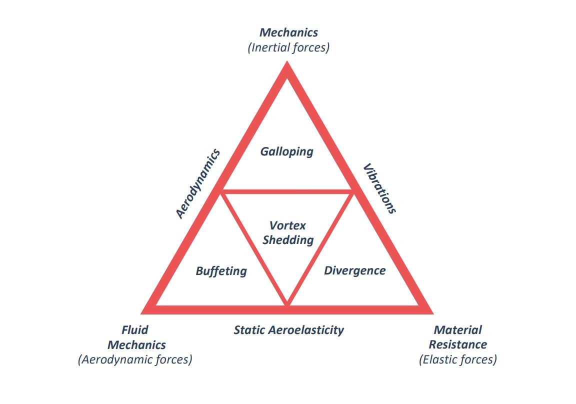
Vortex shedding on solar trackers
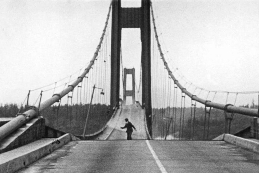
Structural oscillations induced by vortex shedding on solar trackers are due to a vibration effect associated with the vortex street formed in the wake. In a photovoltaic plant, unlike torsional galloping and divergence, vortex shedding occurs over a wide range of wind speeds and, because of the sharp geometry of the tracker section, is inevitable, so the fatigue of the torsion tube section under these oscillatory loads must be taken into account.
It is the responsibility of the aeroelasticity area to define the amplitude and frequency of these oscillations for each wind speed and section inclination to ensure the tracker reliability under these loads.
The Strouhal number (St) describes the frequency at which vortices detach from a body in an oscillatory way, according to the formula:
St = \Large \frac {f L} {U}
Where:
- St: Strouhal number
- f: vortex shedding frequency
- L: characteristic length
- U: fluid speed
Vincenc Strouhal (Čeněk Strouhal)
(Seč, 1850 – Praga, 1922)
Czech physicist specialized in experimental physics. In 1878, while working with cables that experienced vortex shedding and tones in the wind, he defined the Strouhal number (St) that describes oscillating flow mechanisms for fluid-dynamics.
Although there are many studies for cylindrical shapes, especially for chimney designs, where the Strouhal number is related to the Reynolds number to know how the vortex shedding varies with respect to the fluid speed, this is not the case with other surfaces such as a flat plate in similarity with tracker sections. Therefore, the shedding frequencies must be studied for each wind speed and for each tracker tilt to determine if the tracker enters into resonance.
For practical purposes, oscillatory vortex shedding on solar trackers, leeward side, can be considered as an oscillatory moment that is supported by each arm or torque tube on each side of tracker drive system plus a static moment. This oscillatory moment will cause a rotation of the tracker sections whose greatest amplitude will be observed on the farthest from the drive system and tangential stresses in the closest section to the drive on the torque tube in order to support these loads.
Thus, we can express the external moment on the tracker as:
M(t) = M_d sen(\omega t) + M_{est}
Where \omega = 2 \pi f , with f defined in the Strouhal number.
Therefore, we can write the differential equation defining the tracker motion as:
\normalsize I \ddot \theta + 2 I \omega_n \xi \dot \theta + k \theta = M(t) = M_d sen(\omega t) + M_{est}
The complete response of the system to these loads with null initial conditions is as follows:
\normalsize \theta (t) = e^{-\xi \omega_n t} \left[A \cos(\omega_d t) + B sin(\omega_d t)\right] + X sen(\omega t + \phi) + \Large \frac {M_{est}}{k}
Where:
\normalsize X = \Large \frac{M_d/k} {\sqrt{(1-\tau^2)^2 + (2 \xi \tau)^2}}
\phi = \Large \frac{2 \xi \tau} {\sqrt{1-\tau^2}}
A = X sen \phi + \Large \frac{M_{est}} {k}
B = \Large \frac{\xi \omega_n A - X \omega cos \phi}{\omega_d}
\tau = \Large \frac{\omega}{\omega_n}
The expression:
X sen(\omega t + \phi) + \Large \frac {M_{est}}{k}
is called the permanent term and is the solution to the equation when time tends to infinity. The first summand corresponds to the steady response to the oscillatory load, the second one to the static load.
Against, the expression:
e^{-\xi \omega_n t} \left[A \cos(\omega_d t) + B sin(\omega_d t)\right]
is called a transient term and marks the path to the solution until the permanent term is reached.
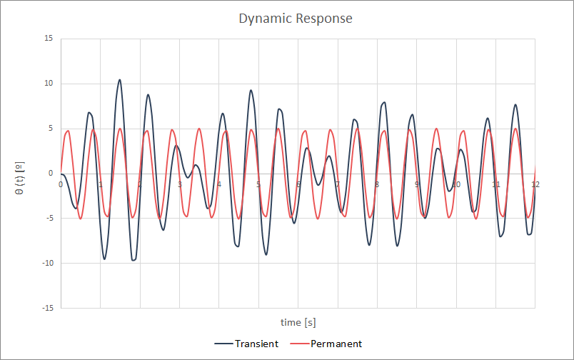
We show some examples of responses to visualize the transient and permanent term.
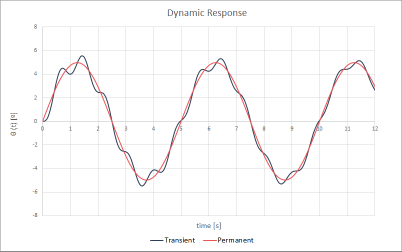
A tracker with an incident oscillatory moment, induced by vortex shedding on the leeward surface, will always tend also to an oscillatory response with the same frequency as the load that excites it, but with a phase shift, and whose amplitude depends on the tracker damping.
On the other hand, if we consider a static load, the response of the tracker will also tend to a constant which, this time, depends on the system stiffness.
Resonance is the vibration phenomenon of a body at the same frequency as the force that excites it. When this occurs, the vibration amplitude of the system is as large as possible and can only be attenuated if there is effective damping.
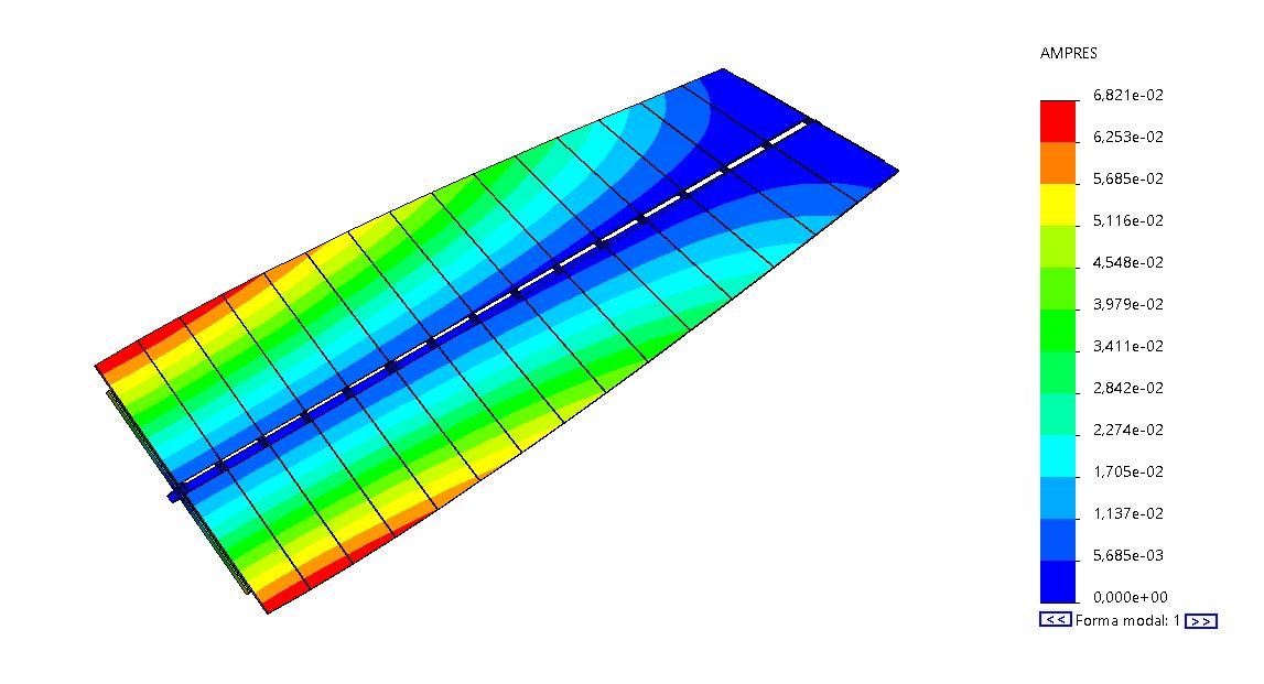
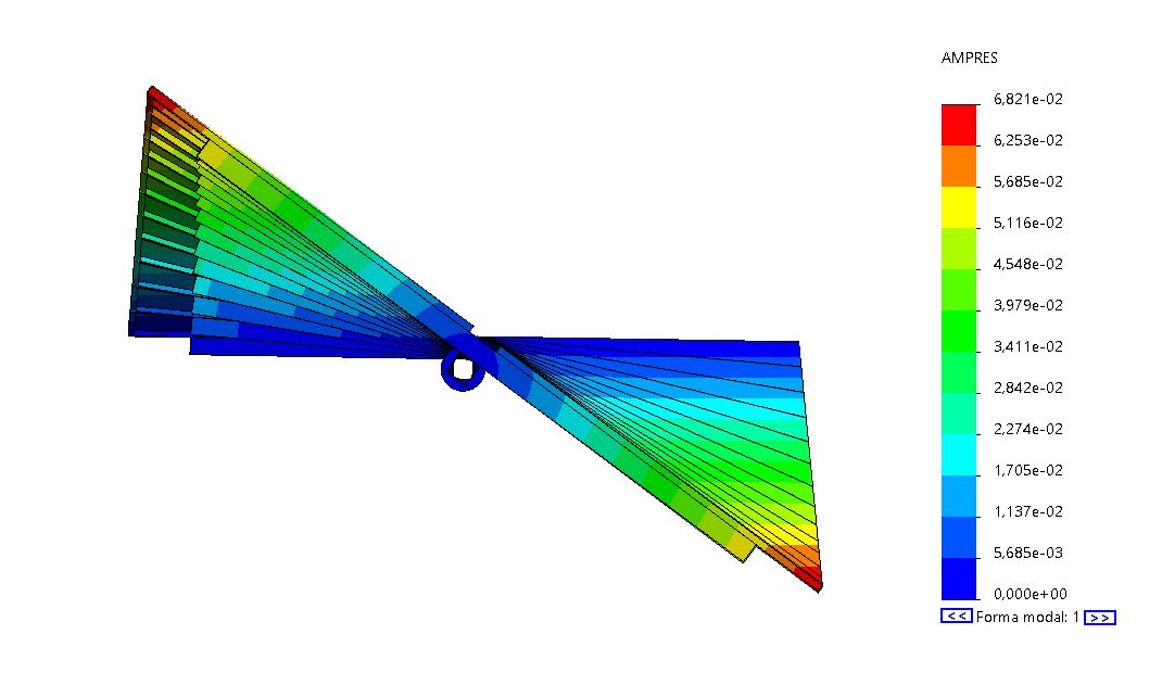
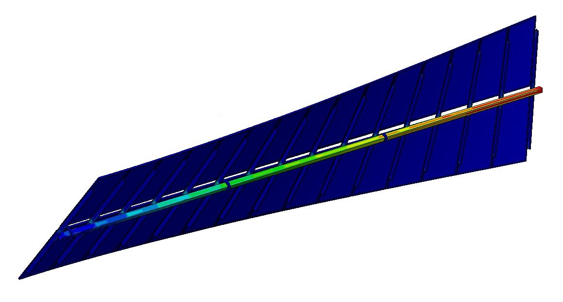
A single-axis solar tracker, like any structure, has several frequencies and associated modes of vibration. If we consider that this tracker has two rows of 15 modules per torque tube, with the torque tube being 17.3m long and #140.5mm in cross section, the first vibration frequency we find is 1.2Hz. Its associated mode of vibration is a torsion along the tracker axis where the largest section twist is found in the section farthest from the drive system (last section).
For simplicity, we will adjust the three-dimensional model to a two-dimensional one with an equivalent inertia (I) and an equivalent stiffness (k) giving the same deformations as the last section in a three-dimensional model for the same state of equivalent loads. For practical purposes, we will assume that the entire tracker deflects and suffers the moments of the section furthest from the drive system. This assumption is on the safety side.
If we consider a tracker whose torsion tube has a square section of 140mm side and 5mm thickness (#140.5) in steel S355JR, the yield limit of this material is reached by means of tangential stresses for combinations of amplitude and frequency of oscillating moments.
The system response is very diverse depending on the proximity of the excitation frequency to the natural frequency and its damping.
Qualitatively, 3 parameters are mainly involved:
The following graph shows the allowed oscillating moments at the yield limit of a #140.5mm torque tube made of steel S355JR for different damping values (ξ). The tracker carries in each torque tube 30 photovoltaic modules arranged in two rows of 15, with a length of 17.3m, a cross section of 4.7m and a natural of 1.2Hz.
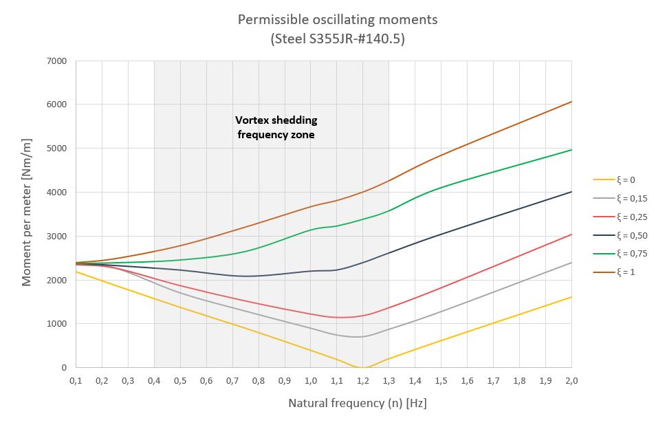
In this section, we are only including the tangential stresses due to torsion ( \tau_t ). Normal stresses due to bending moments ( \sigma_b ) and tangential ones due to shear ( \tau_c ) produced by drag and lift wind loads must be taken into account according to the Von Mises stress ( \sigma_{VM} ) to compute the overall stress on the torque tube.
\sigma_{VM} = \sqrt{\sigma_b^2 + 3 (\tau_t + \tau_c)^2}
The wind stow speed ( U_{stow,3s,10m} ) in photovoltaic plants is usually between 15 and 20 m/s depending on the location. Vortex shedding on solar trackers must be studied for all tracker tilts below this speed. In addition, for the chosen stow position and up to the plant survival speed, the stresses reached on the torque tube due to this phenomenon must be below the yield limit of the material which make it up.
It is important to underline that, for wind speeds close to the plant survival speed, slight tracker tilts for stow position to enhance the effects of galloping can negatively influence the vortex shedding phenomenon. While at high wind speeds the shedding frequencies are usually low and below the system natural frequency, the amplitudes due to the high wind speed are not, as they are directly proportional to the square of the wind speed and can cause significant stresses on the torque tube.
For this reason, and for the stow position, damping must be chosen both to ensure that the galloping critical speed is above the plant survival speed, and to ensure that the vibrations produced by vortex shedding do not provide stresses that exceed the torque tube yield limit before the survival speed is reached.
We have defined the system response to oscillatory moments induced by vortex shedding on solar trackers. The next step is to determine the amplitude and frequency values of these moments for a given wind speed together with a given tracker tilt, since this frequency and amplitude will change due to these two factors.
The system natural frequency (n) given by its stiffness (k) as well as the damping coefficient (ξ) play a very important role, since the tracker will rotate as much as the stiffness allows it for position and damping for velocity, obtaining variable moments which depend on these two values.
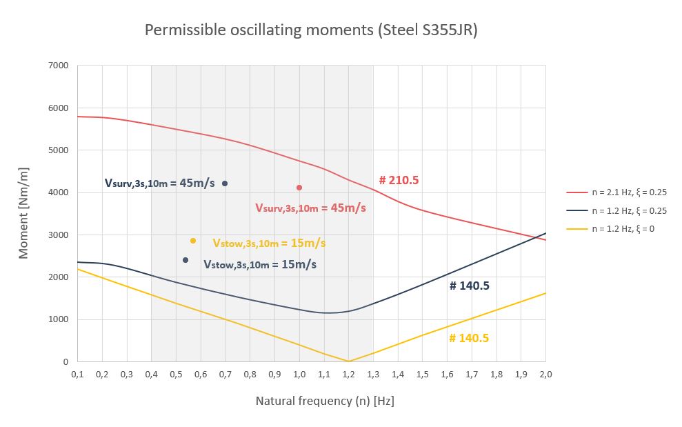
A tracker with a natural frequency of 1.2Hz without physical damping as such cannot withstand the oscillating moments due to the wind that provides the plant survival velocity ( U_{surv,3s,10m} \small \approx 45m/s ), as it will generate strains with too high amplitudes that will cause stresses on the torque tube that exceed its yield limit long before reaching that speed. In fact, it will not do so for any possible damping. To achieve that, it would be necessary to modify the system stiffness by increasing the torque tube cross section to #210.5, thus raising the system natural frequency (n) to 2.1Hz.
Response to any function
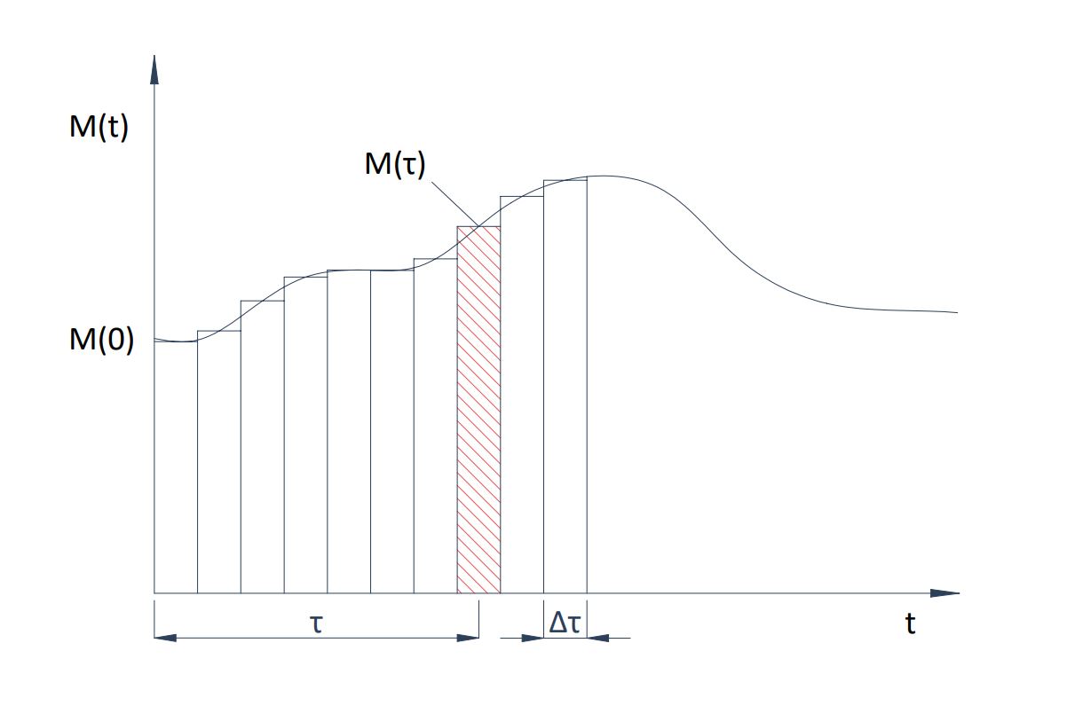
Any external force affecting the tracker can be represented by a function in time that can be approximated by the sum of a series of steps M(\tau) of finite duration \Delta \tau . Each of them produces an impulse of M(\tau) \Delta \tau.
This approximation can be expressed in the form:
M(t) = \sum_{i=1}^n M(\tau_i)
Having a constant value, M(\tau_i), in each interval between \tau_i - \large \frac{\Delta \tau}{2} and \tau_i + \large \frac{\Delta \tau}{2} (equal to the value of the function at point τ_i) and being null for the rest of the time.
If the values of \Delta \tau are made to tend to zero, \Delta \tau \rightarrow d\tau, impulses will have a value M(\tau) d\tau. In this case, the approximation by a sum of infinite impulses becomes exact. The value of the response to each of the impulses in which the function has been divided, for zero initial conditions, can be expressed as:
d\theta(t) = M(\tau) h(t-\tau) d\tau
Where d\theta(t) represents the increase in the response value due to the differential impulse M(\tau) d\tau, and h(t-\tau) is the response value to a unit impulse produced at instant \tau (with zero initial conditions).
Thus, applying the superposition principle, with null initial conditions, the response at any instant t, will be:
\theta(t) = \large \int_0^t \normalsize M(\tau) h(t-\tau) d\tau
Expression called Duhamel integral.
Jean-Marie Constante Duhamel
(Saint-Malo, 1797 – París, 1872)
French mathematician and physicist who made notable contributions to infinitesimal calculus. Duhamel’s theorem applied to infinitesimal calculus states that the sum of a series of infinitesimals is maintained when they are replaced by their principal part.
The function h(t-\tau), impulse response at instant t-\tau, can be expressed by:
h(t-\tau) = \Large \frac{e^{-\xi \omega_n (t-\tau)}}{I\omega_d} \normalsize \sin \left[ \omega_d(t-\tau)\right]
According to these expressions and taking into account zero initial conditions, the response in time of a one degree of freedom system, forced to any function M(t), can be obtained by the equation:
\theta(t) = \large \int_0^t \normalsize M(\tau) \Large \frac{e^{-\xi \omega_n (t-\tau)}}{I\omega_d} \normalsize \sin \left[ \omega_d(t-\tau)\right] d\tau
Taking into account that it is integrated over \tau, so that t is constant, and considering the sine of angles that are subtracted, we have that:
\theta(t) = \Large \frac{e^{-\xi \omega_n t}}{I\omega_d} \normalsize \left[ C1 \sin(\omega_dt) - C2 \cos(\omega_dt)\right]
Where:
C1 = \large \int_0^t \normalsize M(\tau) e^{ \xi \omega_n \tau} \cos( \omega_d\tau) d\tau
C2 = \large \int_0^t \normalsize M(\tau) e^{ \xi \omega_n \tau} \sin( \omega_d\tau) d\tau
Deriving the above expression with respect to time (t) results in the expression for the vibration velocity of the tracker:
\dot \theta(t) = \Large \frac{d\theta(t)}{dt} \normalsize = \Large \frac{e^{-\xi \omega_n t}}{I\omega_d} \normalsize (A1 + A2 )
With A1 y A2 as:
A1 = C1 \left[ -\xi \omega_n \sin(\omega_dt) + \omega_d \cos(\omega_dt)\right]
A2 = C2 \left[ \xi \omega_n \cos(\omega_dt) + \omega_d \sin(\omega_dt)\right]
These two integrals, C1 and C2, can be approximated through any numerical method of integration. For trapezoidal rule, we have that:
\large \int_a^b \normalsize f(x) dx \approx \Large \frac{b-a}{2} \normalsize \left[ f(a) + f(b) \right]
And since a computer software divides the time into very small intervals and calculates a solution at each interval, we can approximate the integrals as follows:
\small C1(t) \approx C1(t-1) + \normalsize \frac{\Delta t}{2} \small \left[ M(t) e^{ \xi \omega_n t}\cos(\omega_dt) + M(t-1) e^{ \xi \omega_n (t-1)}\cos(\omega_d(t-1)) \right]
\small C2(t) \approx C2(t-1) + \normalsize \frac{\Delta t}{2} \small \left[ M(t) e^{ \xi \omega_n t}\sin(\omega_dt) + M(t-1) e^{ \xi \omega_n (t-1)}\sin(\omega_d(t-1)) \right]
Vortex shedding + Galopping/Divergence
Due mainly to the sharp shape of the tracker sections, vortex shedding on solar trackers will be present in solar plants as long as the wind blows with a considerable speed, therefore, stiffness (k) and damping (ξ) of the system should be designed to minimize the tangential stresses in the torsion tube.
Torsional galloping and divergence appear at a given and specific wind speed. If stiffness and damping values of trackers are well dimensioned, these two phenomena will appear beyond the survival speed of the plant and should not be considered together with vortex shedding, since they would be independent phenomena and would never appear at the same time.
In the event of such a situation, galloping or divergence provide much stronger instabilities than vortex shedding on solar trackers, only comparable to the latter if vortex shedding occurred at resonance ( \omega = \omega_n ) with zero damping ( \xi \approx 0 ). Thus, catastrophic failure in tracker is considered if they come into:
Related posts
Projects


About us